Creating a pool set for matchRanges

Introduction

matchRanges() performs subset selection on a pool of ranges such that chosen covariates are distributionally matched to a focal set of ranges. However, the generation of a set of pool ranges is not a trivial task. This vignette provides some guidance for how to generate a pool of ranges.

For this analysis, we use DNase peaks as a measure of open chromatin, and ChIP-seq for JUN peaks as a measure of JUN binding. Suppose we are interested in the properties of chromatin accessibility, but suspect that JUN-binding impacts accessibility. We can use matchRanges() to control for the DNase signal and the length of the site so we can compare our JUN-bound sites (i.e., our focal set) to sites where JUN is not bound (i.e., our pool set).

Obtaining example data

First, we use AnnotationHub to access GRanges for DNase and JUN narrowPeaks in human (hg19) GM12878 cells:

library(AnnotationHub)
ah <- AnnotationHub()

dnase <- ah[["AH30743"]]
junPeaks <- ah[["AH22814"]]

dnase

## GRanges object with 271214 ranges and 6 metadata columns:
##            seqnames              ranges strand |        name     score
##               <Rle>           <IRanges>  <Rle> | <character> <numeric>
##        [1]     chrM              1-1096      * |      Rank_1      2806
##        [2]     chrM           1210-4181      * |      Rank_2      2806
##        [3]     chrM          8868-16581      * |      Rank_3      2806
##        [4]     chrM           4661-5575      * |      Rank_4      2784
##        [5]    chr21     9825397-9827624      * |      Rank_5      2741
##        ...      ...                 ...    ... .         ...       ...
##   [271210]     chr2   99101766-99101877      * | Rank_271210        20
##   [271211]     chr6       319032-319131      * | Rank_271211        20
##   [271212]     chr1 117329477-117329556      * | Rank_271212        20
##   [271213]     chr1   45985571-45985660      * | Rank_271213        20
##   [271214]     chr2 101185965-101186044      * | Rank_271214        20
##            signalValue    pValue    qValue      peak
##              <numeric> <numeric> <numeric> <numeric>
##        [1]     76.6491   280.660   271.178       485
##        [2]     76.6491   280.660   271.178      2340
##        [3]     76.6491   280.660   271.178      5029
##        [4]     76.1730   278.495   271.178       288
##        [5]     75.2208   274.173   268.040       814
##        ...         ...       ...       ...       ...
##   [271210]     2.15692   2.00390   0.46416        71
##   [271211]     2.15692   2.00390   0.46416        40
##   [271212]     2.19528   2.00202   0.46235        43
##   [271213]     2.19528   2.00202   0.46235        42
##   [271214]     2.19528   2.00202   0.46235        26
##   -------
##   seqinfo: 298 sequences (2 circular) from hg19 genome

Since we want to control for accessibility, we can use the signalValue from the DNase peaks as a covariate. DNase sites are also different lengths. If we suspect length might impact accessibility differently at JUN-bound sites, we can include it as a covariate as well. For visualization, let’s convert these to log-scale using mutate() from plyranges:

library(plyranges)
dnase <- dnase |>
  mutate(log10_signal = log10(signalValue + 1),
         log10_length = log10(width(dnase) + 1))

Creating the `focal` and `pool` sets

Next we define our focal and pool sets. The focal set contains the feature of interest (i.e., DNase peaks bound by JUN), whereas the pool set lacks this feature (i.e., unbound DNase peaks). matchRanges() is designed to handle datasets that can be binarized into these two distinct groups. With plyranges it is easy to filter DNase sites by overlap (or lack of overlap) with JUN peaks:

## Define focal and pool
focal <- dnase |>
  filter_by_overlaps(junPeaks)

pool <- dnase |>
  filter_by_non_overlaps(junPeaks)

The focal set must be smaller than the pool set for matching to work correctly. Matching is most effective when the pool set is much larger and covers all values in the focal set.

length(focal)

## [1] 2490

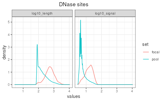
length(pool)

## [1] 268724

length(pool)/length(focal)

## [1] 107.9213

Before matching, the focal set shows a different distribution of length and signal than the pool set:

## Before matching, focal shows higher
## signalValue than pool
library(tidyr)
library(ggplot2)
bind_ranges(focal=focal,
            pool=pool,
            .id="set") |>
  as.data.frame() |>
  pivot_longer(cols=c("log10_length", "log10_signal"),
               names_to="features",
               values_to="values") |>
  ggplot(aes(values, color=set)) +
  facet_wrap(~features) +
  stat_density(geom='line', position='identity') +
  ggtitle("DNase sites") +
  theme_bw() +
  theme(plot.title=element_text(hjust=0.5))

Obtaining the matched set with `matchRanges()`

To control for these differences, we can use matchRanges() to select a subset of unbound DNase sites from the pool that have the same distribution of length and signal.

library(nullranges)
set.seed(123)
mgr <- matchRanges(focal=focal,
                   pool=pool,
                   covar=~log10_length + log10_signal,
                   method='rejection',
                   replace=FALSE)

mgr

## MatchedGRanges object with 2490 ranges and 8 metadata columns:
##          seqnames              ranges strand |        name     score
##             <Rle>           <IRanges>  <Rle> | <character> <numeric>
##      [1]    chr13   42242369-42242758      * |  Rank_13919       498
##      [2]     chr4 148721069-148721751      * |   Rank_6820       733
##      [3]     chr1 167522710-167523305      * |   Rank_8764       655
##      [4]    chr22   36771568-36771911      * |  Rank_61304       119
##      [5]    chr12   27863138-27864123      * |   Rank_9430       628
##      ...      ...                 ...    ... .         ...       ...
##   [2486]     chr1 236311692-236312194      * |  Rank_31397       247
##   [2487]     chr9 135257201-135258016      * |  Rank_10743       592
##   [2488]     chr6     2842064-2842353      * |  Rank_46877       165
##   [2489]    chr11     1542262-1543612      * |   Rank_9405       628
##   [2490]     chr7   90561352-90561734      * |  Rank_44121       176
##          signalValue    pValue    qValue      peak log10_signal log10_length
##            <numeric> <numeric> <numeric> <numeric>    <numeric>    <numeric>
##      [1]    19.99541   49.8679  46.71972       107     1.322124      2.59218
##      [2]    21.33174   73.3284  69.75892       208     1.348923      2.83506
##      [3]    22.83272   65.5173  62.09552       349     1.377174      2.77597
##      [4]     7.14122   11.9399   9.63032       258     0.910689      2.53782
##      [5]    23.80406   62.8724  59.48975       599     1.394523      2.99432
##      ...         ...       ...       ...       ...          ...          ...
##   [2486]    10.63635   24.7928   22.1325       223     1.065817      2.70243
##   [2487]    19.80561   59.2923   55.9855       398     1.318180      2.91222
##   [2488]     8.06895   16.5491   14.1081        93     0.957557      2.46389
##   [2489]    23.80406   62.8724   59.4898       968     1.394523      3.13098
##   [2490]     8.43572   17.6751   15.2014       173     0.974775      2.58433
##   -------
##   seqinfo: 298 sequences (2 circular) from hg19 genome

Assessing covariate balance

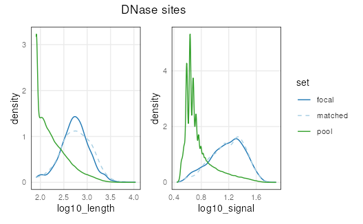
Now let’s use the plotCovariate() function with patchwork to visualize how similar our matched distribution is to focal:

library(patchwork)
lapply(covariates(mgr),
       plotCovariate,
       x=mgr,
       sets=c('f', 'm', 'p')) |>
  Reduce('+', x=_) +
  plot_layout(guides="collect") +
  plot_annotation(title="DNase sites",
                  theme=theme(plot.title=element_text(hjust=0.40)))

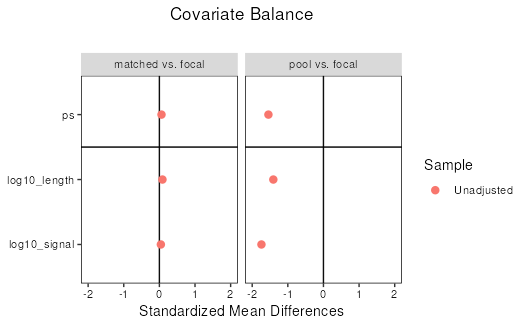
An important part of propensity-score matching, is assessing similarity, or balance, between the focal and matched sets. One way is to visually examine the distributions as we have done above. Another way is to report summary statistics about the two sets. cobalt is a package designed to specifically address covariate balance after covariate matching. Below, we demonstrate how to use cobalt to calculate the standardized mean differences and visualize these statistics with a love plot. For more information about assessing covariate balance, refer to the detailed documentation in the cobalt vignette: vignette("cobalt", package = "cobalt").

library(cobalt)
res <- bal.tab(f.build("set", covariates(mgr)),
               data=matchedData(mgr)[!set %in% 'unmatched'],
               distance="ps",
               focal="focal",
               which.treat="focal",
               s.d.denom="all")

res

## Balance by treatment pair
## 
##  - - - focal (0) vs. matched (1) - - - 
## Balance Measures
##                  Type Diff.Un
## ps           Distance  0.0594
## log10_length  Contin.  0.0862
## log10_signal  Contin.  0.0415
## 
## Sample sizes
##     focal matched
## All  2490    2490
## 
##  - - - focal (0) vs. pool (1) - - - 
## Balance Measures
##                  Type Diff.Un
## ps           Distance -1.5447
## log10_length  Contin. -1.4070
## log10_signal  Contin. -1.7405
## 
## Sample sizes
##     focal   pool
## All  2490 268724
##  - - - - - - - - - - - - - - - - - - - - - - - - -

plot(res) + xlim(c(-2, 2))

The “focal vs. matched” comparison shows much lower standardized mean differences than “focal vs. pool”, indicating that the matched set has been successfully controlled for covariates of DNAse site length and signal.

Eric S. Davis

08/21/2023

Introduction

Obtaining example data

Creating the `focal` and `pool` sets

Obtaining the matched set with `matchRanges()`

Assessing covariate balance

Creating a pool set for matchRanges

Eric S. Davis

08/21/2023

Introduction

Obtaining example data

Creating the focal and pool sets

Obtaining the matched set with matchRanges()

Assessing covariate balance

Creating the `focal` and `pool` sets

Obtaining the matched set with `matchRanges()`