Matching case study II: CTCF orientation
Eric S. Davis
11/20/2025
Source:vignettes/matching_ginteractions.Rmd
matching_ginteractions.RmdIn this vignette, we demonstrate the generation of covariate-matched
null ranges by using the matchRanges() function to test the
“covergence rule” of CTCF-bound chromatin loops, first described in Rao
et al. 2014.
Background
In the human genome, chromatin loops play an important role in regulating gene expression by connecting regulatory loci to gene promoters. The anchors of these loops are bound by the protein CTCF, which is required for loop formation and maintenance. CTCF binds a specific non-palindromic DNA sequence motif. And the direction of this motif at loop anchors is non-random. That is, CTCF binding motifs found at the anchors of loops tend to be oriented towards the center of the loop more often then would be expected by chance. This phenomenon, first described by Rao et al in 2014, is known as the “convergence rule”. It was initially discovered by first filtering for loops that had a single CTCF binding site at each end of the loop. Here we use matchRanges to reinvestigate the convergence using all loops.
We will use hg19_10kb_ctcfBoundBinPairs data from the
nullrangesData package which contains features from the
GM12878 cell line aligned to hg19 as well as CTCF motif data from the CTCF
data package available on Bioconductor.
hg19_10kb_ctcfBoundBinPairs is a GInteractions
object with all pairwise combinations of CTCF-bound 10Kb bins within 1Mb
annotated with the following features:
- The total CTCF signal in each bin.
- The number of CTCF sites in each bin.
- The distance between bin pairs.
- Whether at least one CTCF site is convergent between each bin pair.
- The presence or absence of a loop between each bin pair.
Using these annotations and the matchRanges() function,
we can compare CTCF motif orientations between pairs of genomic regions
that are 1) connected by loops, 2) not connected by loops, 3) randomly
chosen, or 4) not connected by loops, but matched for the strength of
CTCF sites and distance between loop anchors.
Matching with matchRanges()
Before we generate our null ranges, let’s take a look at our example dataset:
library(nullrangesData)
## Load example data
binPairs <- hg19_10kb_ctcfBoundBinPairs()
binPairs
## StrictGInteractions object with 198120 interactions and 5 metadata columns:
## seqnames1 ranges1 seqnames2 ranges2 |
## <Rle> <IRanges> <Rle> <IRanges> |
## [1] chr1 230001-240000 --- chr1 520001-530000 |
## [2] chr1 230001-240000 --- chr1 710001-720000 |
## [3] chr1 230001-240000 --- chr1 800001-810000 |
## [4] chr1 230001-240000 --- chr1 840001-850000 |
## [5] chr1 230001-240000 --- chr1 870001-880000 |
## ... ... ... ... ... ... .
## [198116] chrX 154310001-154320000 --- chrX 154370001-154380000 |
## [198117] chrX 154310001-154320000 --- chrX 155250001-155260000 |
## [198118] chrX 154320001-154330000 --- chrX 154370001-154380000 |
## [198119] chrX 154320001-154330000 --- chrX 155250001-155260000 |
## [198120] chrX 154370001-154380000 --- chrX 155250001-155260000 |
## looped ctcfSignal n_sites distance convergent
## <logical> <numeric> <factor> <integer> <logical>
## [1] FALSE 5.18038 2 290000 FALSE
## [2] FALSE 5.46775 2 480000 TRUE
## [3] FALSE 7.30942 2 570000 FALSE
## [4] FALSE 7.34338 2 610000 FALSE
## [5] FALSE 6.31338 3 640000 TRUE
## ... ... ... ... ... ...
## [198116] FALSE 6.79246 2 60000 FALSE
## [198117] FALSE 6.12447 3 940000 TRUE
## [198118] FALSE 7.40868 2 50000 TRUE
## [198119] FALSE 7.00936 3 930000 FALSE
## [198120] FALSE 6.73402 3 880000 TRUE
## -------
## regions: 20612 ranges and 5 metadata columns
## seqinfo: 23 sequences from hg19 genomeLet’s start by defining our focal set (i.e. looped bin-pairs), our
pool set (i.e un-looped bin-pairs), and our covariates of interest
(i.e. ctcfSignal and distance):
library(nullranges)
set.seed(123)
mgi <- matchRanges(focal = binPairs[binPairs$looped],
                   pool = binPairs[!binPairs$looped],
                   covar = ~ctcfSignal + distance + n_sites,
                   method = 'stratified')
mgi
## MatchedGInteractions object with 3104 interactions and 5 metadata columns:
## seqnames1 ranges1 seqnames2 ranges2 |
## <Rle> <IRanges> <Rle> <IRanges> |
## [1] chr11 62160001-62170000 --- chr11 62190001-62200000 |
## [2] chr17 7890001-7900000 --- chr17 7990001-8000000 |
## [3] chr22 36460001-36470000 --- chr22 36680001-36690000 |
## [4] chr11 1560001-1570000 --- chr11 1710001-1720000 |
## [5] chr19 17880001-17890000 --- chr19 17960001-17970000 |
## ... ... ... ... ... ... .
## [3100] chr7 25100001-25110000 --- chr7 25220001-25230000 |
## [3101] chr19 14310001-14320000 --- chr19 14540001-14550000 |
## [3102] chr11 6010001-6020000 --- chr11 6300001-6310000 |
## [3103] chr6 37450001-37460000 --- chr6 37620001-37630000 |
## [3104] chr11 1840001-1850000 --- chr11 2170001-2180000 |
## looped ctcfSignal n_sites distance convergent
## <logical> <numeric> <factor> <integer> <logical>
## [1] FALSE 8.12860 2 30000 FALSE
## [2] FALSE 8.72976 3 100000 TRUE
## [3] FALSE 9.51410 4 220000 TRUE
## [4] FALSE 8.64759 3 150000 FALSE
## [5] FALSE 8.52097 2 80000 FALSE
## ... ... ... ... ... ...
## [3100] FALSE 7.87730 2 120000 FALSE
## [3101] FALSE 8.13800 2 230000 FALSE
## [3102] FALSE 7.05064 2 290000 FALSE
## [3103] FALSE 8.72932 4 170000 TRUE
## [3104] FALSE 8.39022 3 330000 TRUE
## -------
## regions: 20612 ranges and 5 metadata columns
## seqinfo: 23 sequences from hg19 genomeWhen the focal and pool arguments are GInteractions
objects, matchRanges() returns a
MatchedGInteractions object. The
MatchedGInteractions class extends
GInteractions so all of the same operations can be
applied:
library(plyranges)
library(ggplot2)
## Summarize ctcfSignal by n_sites
mgi %>%
  regions() %>%
  group_by(n_sites) %>%
  summarize(ctcfSignal = mean(ctcfSignal)) %>%
  as.data.frame() %>%
  ggplot(aes(x = n_sites, y = ctcfSignal)) +
    geom_line() +
    geom_point(shape = 21, stroke = 1,  fill = 'white') +
    theme_minimal() +
    theme(panel.border = element_rect(color = 'black',
                                      fill = NA))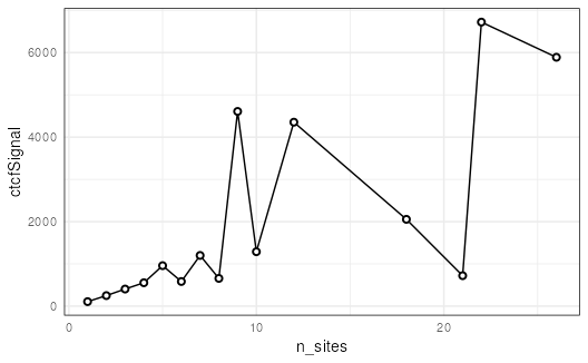
Assessing quality of matching
We can get a quick summary of the matching quality with
overview():
ov <- overview(mgi)
ov
## MatchedGInteractions object:
## set N ctcfSignal.mean ctcfSignal.sd distance.mean distance.sd
## <char> <num> <num> <num> <num> <num>
## focal 3104 8.3 0.67 320000 230000
## matched 3104 8.3 0.69 320000 250000
## pool 195016 7.9 0.85 490000 290000
## unmatched 191928 7.8 0.85 490000 290000
## n_sites.0 n_sites.1 n_sites.2 n_sites.3 n_sites.4 n_sites.5 n_sites.6
## <num> <num> <num> <num> <num> <num> <num>
## 0 0 2167 734 164 32 4
## 0 0 2212 702 150 34 4
## 0 0 152318 34992 5971 944 158
## 0 0 150122 34290 5821 910 154
## n_sites.7+ ps.mean ps.sd
## <num> <num> <num>
## 3 0.026 0.016
## 2 0.026 0.016
## 633 0.016 0.013
## 631 0.015 0.013
## --------
## focal - matched:
## ctcfSignal.mean ctcfSignal.sd distance.mean distance.sd n_sites.0 n_sites.1
## <num> <num> <num> <num> <num> <num>
## 0.0014 -0.029 -1300 -27000 0 0
## n_sites.2 n_sites.3 n_sites.4 n_sites.5 n_sites.6 n_sites.7+ ps.mean ps.sd
## <num> <num> <num> <num> <num> <num> <num> <num>
## -45 32 14 -2 0 1 -7.2e-08 -4.4e-07In addition to providing a printed overview, the overview data can be
extracted for convenience. For example, the quality
property shows the absolute value of the mean difference between focal
and matched sets. Therefore, the lower this value, the better the
matching quality:
ov$quality## [1] 7.2e-08Visualizing matching results
Let’s visualize overall matching quality by plotting propensity scores for the focal, pool, and matched sets:
plotPropensity(mgi, sets = c('f', 'p', 'm'))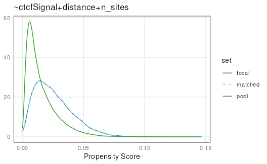
Log transformations can be applied to ‘x’, ‘y’, or both
(c('x', 'y')) for plotting functions to make it easier to
assess quality. It is clear that the matched set is very well matched to
the focal set:
plotPropensity(mgi, sets = c('f', 'p', 'm'), log = 'x')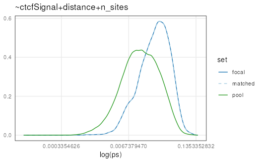
We can ensure that covariate distributions have been matched
appropriately by using the covariates() function to extract
matched covariates along with patchwork and
plotCovarite to visualize all distributions:
library(patchwork)
plots <- lapply(covariates(mgi), plotCovariate, x=mgi, sets = c('f', 'm', 'p'))
Reduce('/', plots)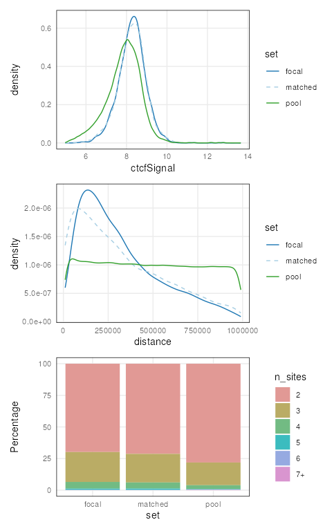
Compare CTCF site orientation
Using our matched ranges, we can compare the percent of looped pairs
with at least one convergent CTCF site against unlooped pairs, randomly
selected pairs, and pairs that are unlooped but have been matched for
our covariates. The accessor function focal() and
pool() can be used to conveniently extract these matched
sets:
## Generate a randomly selected set from all binPairs
all <- c(focal(mgi), pool(mgi))
set.seed(123)
random <- all[sample(1:length(all), length(mgi), replace = FALSE)]
## Calculate the percent of convergent CTCF sites for each group
g1 <- (sum(focal(mgi)$convergent) / length(focal(mgi))) * 100
g2 <- (sum(pool(mgi)$convergent) / length(pool(mgi))) * 100
g3 <- (sum(random$convergent) / length(random)) * 100
g4 <- (sum(mgi$convergent) / length(mgi)) * 100
## Visualize
barplot(height = c(g1, g2, g3, g4),
        names.arg = c('looped\n(focal)', 'unlooped\n(pool)',
                      'all pairs\n(random)', 'unlooped\n(matched)'),
        col = c('#1F78B4', '#33A02C', 'orange2', '#A6CEE3'),
        ylab = "Convergent CTCF Sites (%)",
        main = "Testing the Convergence Rule",
        border = NA,
        las = 1)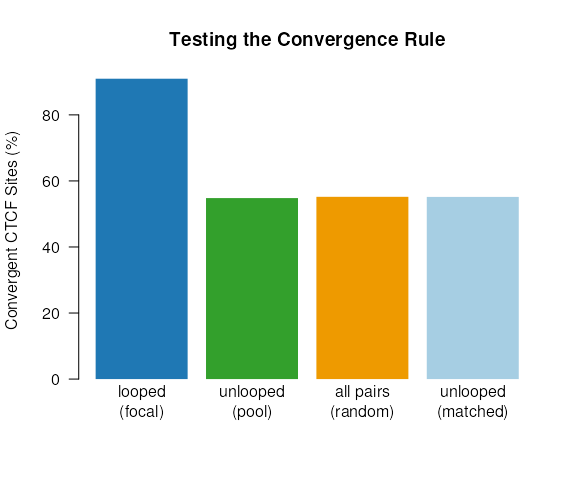
As shown above the convergent rule holds true even when controlling for CTCF signal strength and bin pair distance. Greater than 90% of looped pairs contain convergent CTCF sites, compared to only ~55% among non-looped subsets.
Session information
## R version 4.5.2 (2025-10-31)
## Platform: x86_64-pc-linux-gnu
## Running under: Ubuntu 24.04.3 LTS
##
## Matrix products: default
## BLAS:   /usr/lib/x86_64-linux-gnu/openblas-pthread/libblas.so.3
## LAPACK: /usr/lib/x86_64-linux-gnu/openblas-pthread/libopenblasp-r0.3.26.so;  LAPACK version 3.12.0
##
## locale:
##  [1] LC_CTYPE=en_US.UTF-8       LC_NUMERIC=C
##  [3] LC_TIME=en_US.UTF-8        LC_COLLATE=en_US.UTF-8
##  [5] LC_MONETARY=en_US.UTF-8    LC_MESSAGES=en_US.UTF-8
##  [7] LC_PAPER=en_US.UTF-8       LC_NAME=C
##  [9] LC_ADDRESS=C               LC_TELEPHONE=C
## [11] LC_MEASUREMENT=en_US.UTF-8 LC_IDENTIFICATION=C
##
## time zone: UTC
## tzcode source: system (glibc)
##
## attached base packages:
## [1] stats4    stats     graphics  grDevices utils     datasets  methods
## [8] base
##
## other attached packages:
##  [1] patchwork_1.3.2             ggplot2_4.0.1
##  [3] plyranges_1.30.1            dplyr_1.1.4
##  [5] nullranges_1.17.3           nullrangesData_1.16.0
##  [7] InteractionSet_1.38.0       SummarizedExperiment_1.40.0
##  [9] Biobase_2.70.0              MatrixGenerics_1.22.0
## [11] matrixStats_1.5.0           GenomicRanges_1.62.0
## [13] Seqinfo_1.0.0               IRanges_2.44.0
## [15] S4Vectors_0.48.0            ExperimentHub_3.0.0
## [17] AnnotationHub_4.0.0         BiocFileCache_3.0.0
## [19] dbplyr_2.5.1                BiocGenerics_0.56.0
## [21] generics_0.1.4
##
## loaded via a namespace (and not attached):
##  [1] DBI_1.2.3                bitops_1.0-9             httr2_1.2.1
##  [4] rlang_1.1.6              magrittr_2.0.4           ggridges_0.5.7
##  [7] compiler_4.5.2           RSQLite_2.4.4            png_0.1-8
## [10] systemfonts_1.3.1        vctrs_0.6.5              pkgconfig_2.0.3
## [13] crayon_1.5.3             fastmap_1.2.0            XVector_0.50.0
## [16] labeling_0.4.3           Rsamtools_2.26.0         rmarkdown_2.30
## [19] ragg_1.5.0               purrr_1.2.0              bit_4.6.0
## [22] xfun_0.54                cachem_1.1.0             cigarillo_1.0.0
## [25] jsonlite_2.0.0           progress_1.2.3           blob_1.2.4
## [28] DelayedArray_0.36.0      BiocParallel_1.44.0      prettyunits_1.2.0
## [31] parallel_4.5.2           R6_2.6.1                 bslib_0.9.0
## [34] RColorBrewer_1.1-3       rtracklayer_1.70.0       jquerylib_0.1.4
## [37] Rcpp_1.1.0               knitr_1.50               Matrix_1.7-4
## [40] tidyselect_1.2.1         abind_1.4-8              yaml_2.3.10
## [43] codetools_0.2-20         curl_7.0.0               lattice_0.22-7
## [46] tibble_3.3.0             withr_3.0.2              KEGGREST_1.50.0
## [49] S7_0.2.1                 evaluate_1.0.5           desc_1.4.3
## [52] Biostrings_2.78.0        pillar_1.11.1            BiocManager_1.30.27
## [55] filelock_1.0.3           RCurl_1.98-1.17          BiocVersion_3.22.0
## [58] hms_1.1.4                scales_1.4.0             glue_1.8.0
## [61] tools_4.5.2              BiocIO_1.20.0            data.table_1.17.8
## [64] GenomicAlignments_1.46.0 fs_1.6.6                 XML_3.99-0.20
## [67] grid_4.5.2               AnnotationDbi_1.72.0     restfulr_0.0.16
## [70] cli_3.6.5                rappdirs_0.3.3           textshaping_1.0.4
## [73] S4Arrays_1.10.0          gtable_0.3.6             sass_0.4.10
## [76] digest_0.6.39            SparseArray_1.10.1       rjson_0.2.23
## [79] htmlwidgets_1.6.4        farver_2.1.2             memoise_2.0.1
## [82] htmltools_0.5.8.1        pkgdown_2.2.0            lifecycle_1.0.4
## [85] httr_1.4.7               bit64_4.6.0-1