Introduction to matchRanges
Eric S. Davis
11/20/2025
Source:vignettes/matchRanges.Rmd
matchRanges.RmdIntroduction
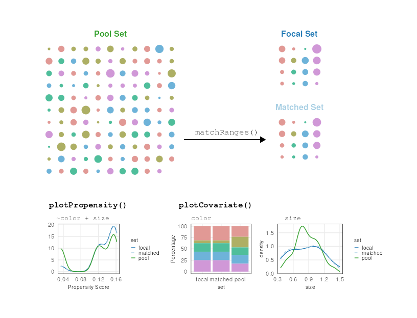
When performing statistical analysis on any set of genomic ranges it
is often important to compare focal sets to null sets that are carefully
matched for possible covariates that may influence the analysis. To
address this need, the nullranges package implements
matchRanges(), an efficient and convenient tool for
selecting a covariate-matched set of null hypothesis ranges from a pool
of background ranges within the Bioconductor framework.
In this vignette, we provide an overview of
matchRanges() and its associated functions. We start with a
simulated example generated with the utility function
makeExampleMatchedDataSet(). We also provide an overview of
the class struture and a guide for choosing among the supported matching
methods. To see matchRanges() used in real biological
examples, visit the Case study I: CTCF
occupancy, and Case study II:
CTCF orientation vignettes.
For a description of the method, see Davis et al. (2023).
Terminology
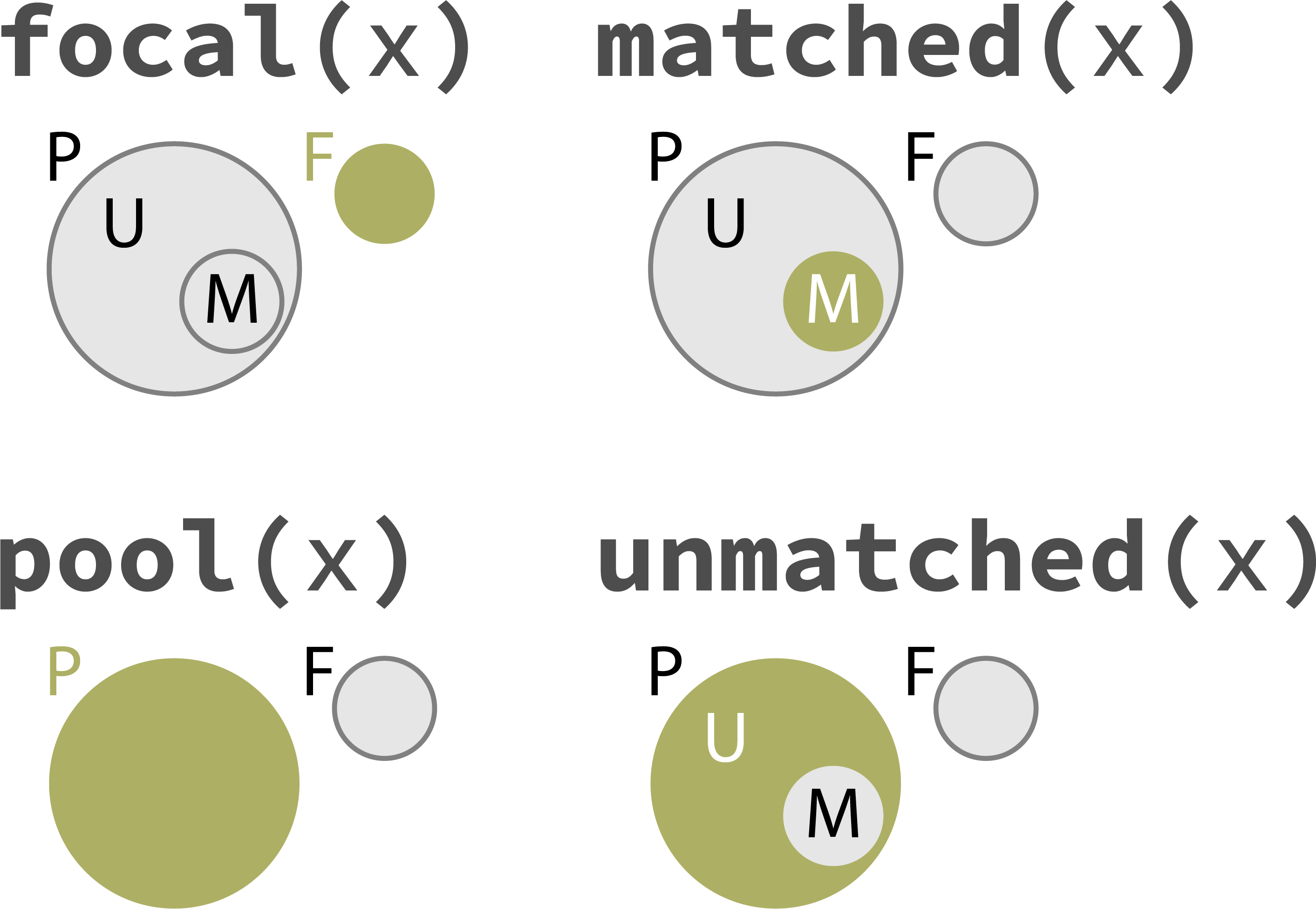
matchRanges references four sets of data:
focal, pool, matched and
unmatched. The focal set contains the outcome
of interest (Y=1) while the pool set contains
all other observations (Y=0). matchRanges
generates the matched set, which is a subset of the
pool that is matched for provided covariates
(i.e. covar) but does not contain the outcome of interest
(i.e Y=0). Finally, the unmatched set contains
the remaining unselected elements from the pool. The
diagram below depicts the relationships between the four sets.
Methodology
matchRanges uses propensity
scores to perform subset selection on the pool set such
that the resulting matched set contains similar
distributions of covariates to that of the focal set. A
propensity score is the conditional probability of assigning an element
(in our case, a genomic range) to a particular outcome (Y)
given a set of covariates. Propensity scores are estimated using a
logistic regression model where the outcome Y=1 for
focal and Y=0 for pool, over the
provided covariates covar. The resulting propensity scores
are used to select matches using one of three available matching
options: “nearest”, “rejection”, or “stratified” with or without
replacement. For more information see the section on Choosing the method parameter below.
Using matchRanges()
We will use a simulated data set to demonstrate matching across covarying features:
library(nullranges)
set.seed(123)
x <- makeExampleMatchedDataSet(type = 'GRanges')
x
## GRanges object with 10500 ranges and 3 metadata columns:
## seqnames ranges strand | feature1 feature2 feature3
## <Rle> <IRanges> <Rle> | <logical> <numeric> <character>
## [1] chr1 1-100 * | TRUE 2.87905 c
## [2] chr1 2-101 * | TRUE 3.53965 c
## [3] chr1 3-102 * | TRUE 7.11742 c
## [4] chr1 4-103 * | TRUE 4.14102 a
## [5] chr1 5-104 * | TRUE 4.25858 c
## ... ... ... ... . ... ... ...
## [10496] chr1 10496-10595 * | FALSE 1.23578 b
## [10497] chr1 10497-10596 * | FALSE 1.69671 a
## [10498] chr1 10498-10597 * | FALSE 6.11140 a
## [10499] chr1 10499-10598 * | FALSE 2.21657 d
## [10500] chr1 10500-10599 * | FALSE 5.33003 b
## -------
## seqinfo: 1 sequence from an unspecified genome; no seqlengthsOur simulated dataset has 3 features: logical feature1,
numeric feature2, and character/factor
feature3. We can use matchRanges() to compare
ranges where feature1 is TRUE to ranges where
feature1 is FALSE, matched by
feature2 and/or feature3:
set.seed(123)
mgr <- matchRanges(focal = x[x$feature1],
                   pool = x[!x$feature1],
                   covar = ~feature2 + feature3)
mgr
## MatchedGRanges object with 500 ranges and 3 metadata columns:
## seqnames ranges strand | feature1 feature2 feature3
## <Rle> <IRanges> <Rle> | <logical> <numeric> <character>
## [1] chr1 8696-8795 * | FALSE 2.87088 c
## [2] chr1 4386-4485 * | FALSE 3.54290 c
## [3] chr1 1094-1193 * | FALSE 7.11436 c
## [4] chr1 5705-5804 * | FALSE 10.78965 b
## [5] chr1 1643-1742 * | FALSE 4.25960 c
## ... ... ... ... . ... ... ...
## [496] chr1 7288-7387 * | FALSE 0.173349 e
## [497] chr1 5539-5638 * | FALSE 4.362421 a
## [498] chr1 8499-8598 * | FALSE 3.182474 e
## [499] chr1 6507-6606 * | FALSE 4.688994 d
## [500] chr1 1860-1959 * | FALSE 5.068635 d
## -------
## seqinfo: 1 sequence from an unspecified genome; no seqlengthsThe resulting MatchedGRanges object is a set of null
hypothesis ranges selected from our pool of options that is
the same length as our input focal ranges and matched for
covar features 2 and 3. These matched ranges print and
behave just as normal GRanges would:
library(GenomicRanges)
sort(mgr)
## MatchedGRanges object with 500 ranges and 3 metadata columns:
## seqnames ranges strand | feature1 feature2 feature3
## <Rle> <IRanges> <Rle> | <logical> <numeric> <character>
## [1] chr1 508-607 * | FALSE 3.54480 c
## [2] chr1 508-607 * | FALSE 3.54480 c
## [3] chr1 510-609 * | FALSE 5.28640 c
## [4] chr1 526-625 * | FALSE 3.82276 a
## [5] chr1 529-628 * | FALSE 3.22564 b
## ... ... ... ... . ... ... ...
## [496] chr1 10414-10513 * | FALSE 9.14097 b
## [497] chr1 10446-10545 * | FALSE 11.23394 e
## [498] chr1 10480-10579 * | FALSE 5.64670 a
## [499] chr1 10483-10582 * | FALSE 3.72415 c
## [500] chr1 10495-10594 * | FALSE 5.37738 b
## -------
## seqinfo: 1 sequence from an unspecified genome; no seqlengthsWe can change the type argument of
makeExampleMatchedDataSet to input data.frames,
data.tables, DataFrames, GRanges and GInteractions objects - all of
which work as inputs for matchRanges. These produce either
MatchedDataFrame, MatchedGRanges, or
MatchedGInteractions objects. For more information about
the Matched class structure and available methods, see the
Class structure section below or the help
documentation for each class, ?MatchedDataFrame,
?MatchedGRanges, or ?MatchedGInteractions.
matchRanges() uses propensity
scores to select matches using one of three available matching
options: “nearest”, “rejection”, or “stratified” with or without
replacement. For more information see the section on Choosing the method parameter below.
Assessing quality of matching
We can assess the quality of Matched classes with
overview(), plotCovariate(), and
plotPropensity(). overview() provides a quick
assessment of overall matching quality by reporting the mean and
standard deviation for covariates and propensity scores of the focal,
pool, matched, and unmatched sets. For factor, character, or logical
covariates (e.g. categorical covariates) the N per set (frequency) is
returned. It also reports the mean difference in focal-matched sets:
overview(mgr)## MatchedGRanges object:
## set N feature2.mean feature2.sd feature3.a feature3.b feature3.c
## <char> <num> <num> <num> <num> <num> <num>
## focal 500 4.1 1.9 66 157 206
## matched 500 4.6 2.7 48 155 223
## pool 10000 6.0 3.4 4248 3121 1117
## unmatched 9559 6.0 3.4 4200 2978 936
## feature3.d feature3.e ps.mean ps.sd
## <num> <num> <num> <num>
## 49 22 0.100 0.076
## 48 26 0.100 0.076
## 992 522 0.045 0.051
## 946 499 0.042 0.048
## --------
## focal - matched:
## feature2.mean feature2.sd feature3.a feature3.b feature3.c feature3.d
## <num> <num> <num> <num> <num> <num>
## -0.48 -0.79 18 2 -17 1
## feature3.e ps.mean ps.sd
## <num> <num> <num>
## -4 -5.8e-06 -6.8e-06Visualizing propensity scores can show how well sets were matched overall:
plotPropensity(mgr)
The distributions of features can be visualized in each set with
plotCovariate():
plotCovariate(mgr)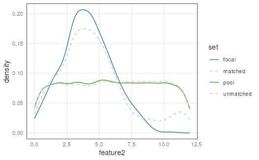
Since these functions return ggplots, patchwork can be
used to visualize all covariates like this:
library(patchwork)
plots <- lapply(covariates(mgr), plotCovariate, x=mgr, sets = c('f', 'm', 'p'))
Reduce('/', plots)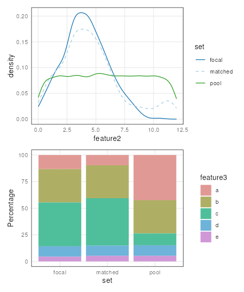
By default, continuous features are plotted as density line plots
while categorical features are plotted as stacked bar plots. All sets
are also shown by default. Defaults can be overridden by setting the
type and sets arguments.
Results from matchRanges can also be used in conjunction
with cobalt for assessing covariate balance. We recommend
using cobalt to calculate and report summary statistics to
indicate adequately matched sets. For more detail on assessing covariate
balance, refer to the detailed documentation on this topic in the
cobalt vignette:
vignette("cobalt", package = "cobalt"). For an example on
how to use cobalt with matchRanges see Using cobalt to assess
balancing.
Accessing matched data
Custom plots can be made by extracting data from the
Matched object:
matchedData(mgr)## Index: <set>
## id feature2 feature3 ps set
## <fctr> <num> <char> <num> <char>
## 1: 1 2.879049 c 0.21095908 focal
## 2: 1 3.539645 c 0.19210984 focal
## 3: 1 7.117417 c 0.11193396 focal
## 4: 1 4.141017 a 0.01771986 focal
## 5: 1 4.258575 c 0.17308581 focal
## ---
## 20555: 0 1.235781 b 0.08945367 unmatched
## 20556: 0 1.696712 a 0.02707977 unmatched
## 20557: 0 6.111404 a 0.01255772 unmatched
## 20558: 0 2.216575 d 0.07578989 unmatched
## 20559: 0 5.330029 b 0.04535856 unmatchedAttributes of the Matched object can be extracted with
the following accessor functions:
covariates(mgr)
method(mgr)
withReplacement(mgr)
## [1] "feature2" "feature3"
## [1] "nearest"
## [1] TRUEEach set can also be extracted with the following accessor functions:
## [1] "GRanges object with 500 ranges and 3 metadata columns"
## [1] "GRanges object with 10000 ranges and 3 metadata columns"
## [1] "GRanges object with 500 ranges and 3 metadata columns"
## [1] "GRanges object with 9559 ranges and 3 metadata columns"
A “tidy” version of key sets can be obtained using plyranges
and the bind_ranges function. This enables efficient
comparisons across sets with other plyranges functionality
(group_by, summarize, etc.).
library(plyranges)
bind_ranges(
  focal = focal(mgr),
  pool = pool(mgr),
  matched = matched(mgr), .id="type"
)
## GRanges object with 11000 ranges and 4 metadata columns:
## seqnames ranges strand | feature1 feature2 feature3 type
## <Rle> <IRanges> <Rle> | <logical> <numeric> <character> <Rle>
## [1] chr1 1-100 * | TRUE 2.87905 c focal
## [2] chr1 2-101 * | TRUE 3.53965 c focal
## [3] chr1 3-102 * | TRUE 7.11742 c focal
## [4] chr1 4-103 * | TRUE 4.14102 a focal
## [5] chr1 5-104 * | TRUE 4.25858 c focal
## ... ... ... ... . ... ... ... ...
## [10996] chr1 7288-7387 * | FALSE 0.173349 e matched
## [10997] chr1 5539-5638 * | FALSE 4.362421 a matched
## [10998] chr1 8499-8598 * | FALSE 3.182474 e matched
## [10999] chr1 6507-6606 * | FALSE 4.688994 d matched
## [11000] chr1 1860-1959 * | FALSE 5.068635 d matched
## -------
## seqinfo: 1 sequence from an unspecified genome; no seqlengthsThe indices() function can be used to find the original
indices for each set. For example,
indices(x, set="matched") will supply the indices from the
pool set that corresponds to the matched set.
In fact, matched(x) is a convenient wrapper around
pool(x)[indices(x, set='matched'):
## [1] TRUEUsing cobalt to assess balancing
This is straight-forward by accessing the data with
matchedData(x):
## cobalt (Version 4.6.1, Build Date: 2025-08-20)
res <- bal.tab(f.build("set", covariates(mgr)),
               data = matchedData(mgr),
               distance = "ps", # name of column containing propensity score
               focal = "focal", # name of focal group in set column
               which.treat = "focal", # compare everything to focal
               s.d.denom = "all") # how to adjust standard deviation

res
## Balance by treatment pair
##
## - - - focal (0) vs. matched (1) - - -
## Balance Measures
## Type Diff.Un
## ps Distance 0.0001
## feature2 Contin. 0.1399
## feature3_a Binary -0.0360
## feature3_b Binary -0.0040
## feature3_c Binary 0.0340
## feature3_d Binary -0.0020
## feature3_e Binary 0.0080
##
## Sample sizes
## focal matched
## All 500 500
##
## - - - focal (0) vs. pool (1) - - -
## Balance Measures
## Type Diff.Un
## ps Distance -1.1274
## feature2 Contin. 0.5523
## feature3_a Binary 0.2928
## feature3_b Binary -0.0019
## feature3_c Binary -0.3003
## feature3_d Binary 0.0012
## feature3_e Binary 0.0082
##
## Sample sizes
## focal pool
## All 500 10000
##
## - - - focal (0) vs. unmatched (1) - - -
## Balance Measures
## Type Diff.Un
## ps Distance -1.1745
## feature2 Contin. 0.5703
## feature3_a Binary 0.3074
## feature3_b Binary -0.0025
## feature3_c Binary -0.3141
## feature3_d Binary 0.0010
## feature3_e Binary 0.0082
##
## Sample sizes
## focal unmatched
## All 500 9559
## - - - - - - - - - - - - - - - - - - - - - - - - - -
love.plot(res)## Warning: Standardized mean differences and raw mean differences are present in
## the same plot. Use the `stars` argument to distinguish between them and
## appropriately label the x-axis. See `?love.plot` for details.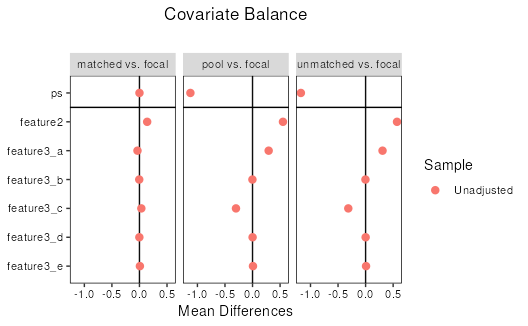
Choosing the method parameter
There are currently 3 available methods for selecting a matched set:
Nearest-neighbor matching with replacement
Rejection sampling with/without replacement
Stratified sampling with/without replacement
Currently, nearest-neighbor matching without replacement is not implemented, but stratified sampling without replacement is a suitable substitute.
Nearest-neighbor matching
Attempts to find the nearest neighbor for each range by using a
rolling-join (as implemented in the data.table package)
between focal and pool propensity scores.
set.seed(123)
mgr <- matchRanges(focal = x[x$feature1],
                   pool = x[!x$feature1],
                   covar = ~feature2 + feature3,
                   method = 'nearest',
                   replace = TRUE)
nn <- overview(mgr)
plotPropensity(mgr)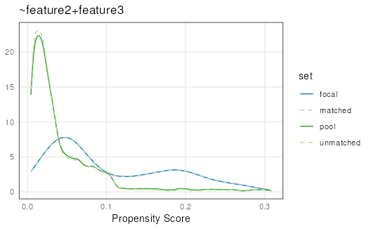
This method is best if you have a very large dataset because it is
usually the fastest matching method. However, because sampling is done
with replacement the user should be careful to assess the number of
duplicate ranges pulled. This can be done using the
indices() function:
## Total number of duplicated indices
length(which(duplicated(indices(mgr))))

sum(table(indices(mgr)) > 1) # used more than once
sum(table(indices(mgr)) > 2) # used more than twice
sum(table(indices(mgr)) > 3) # used more than thrice
## [1] 59
## [1] 51
## [1] 8
## [1] 0Duplicate ranges can be pulled since this method selects the closest matching propensity-score in the focal set to each range in the pool set. It is important to inspect the duplicates when using this method particularly when there are very few well-matching options to select from in your pool set to ensure your matched set has a diverse set of ranges.
Nearest neighbor matching without replacement is not currently supported due to its computational complexity. However, stratified sampling without replacement is an acceptable alternative.
Rejection sampling
Uses a probability-based approach to select options in the
pool that distributionally match the focal set
based on propensity scores. The rejection sampling method first
generates kernal-density estimates for both the focal and pool sets.
Then a scale factor is determined by finding the point at which the
difference in focal and pool densities is maximized. This scale factor
is then applied such that the pool distribution covers the focal
distribution at all points. Random sampling is then conducted, with
probability of accepting a pool range into the matched set given by the
ratio between the height of the density and the scaled (covering)
density. If method or replace is not supplied,
the default values are rejection sampling without replacement.
set.seed(123)
mgr <- matchRanges(focal = x[x$feature1],
                   pool = x[!x$feature1],
                   covar = ~feature2 + feature3,
                   method = 'rejection',
                   replace = FALSE)
rs <- overview(mgr)
plotPropensity(mgr)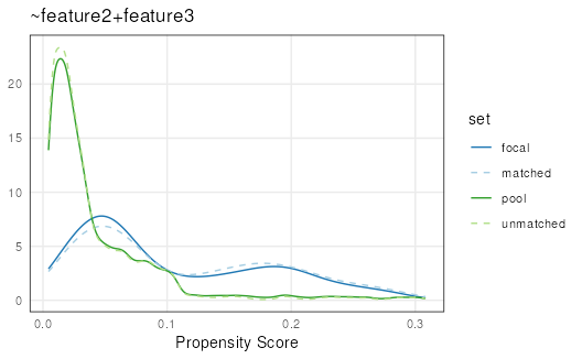
Rejection sampling is the fastest available matching method for sampling without replacement. Therefore, it is ideal to use on large datasets when sampling without replacement is important. However, this method can be unstable, particularly when the pool set is not much larger than the focal set. In those cases, the best method to use is stratified sampling.
Stratified sampling
Performs iterative sampling on increasingly large bins of data.
focal and pool propensity scores are binned by
their value with high granularity, options are randomly selected (with
or without replacement) within each bin and subsequently removed from
the pool of available options. This procedure is repeated, decreasing
the number of bins (and increasing bin size) until the number of
selected matches is equal to the focal set. While matches are being
found in each bin the bins stay small. However, as the number of bins
with no matches increases the algorithm expands bin size faster, which
maintains matching quality while decreasing run-time.
set.seed(123)
mgr <- matchRanges(focal = x[x$feature1],
                   pool = x[!x$feature1],
                   covar = ~feature2 + feature3,
                   method = 'stratified',
                   replace = FALSE)
ss <- overview(mgr)
plotPropensity(mgr)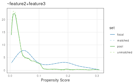
For very large data sets, users might notice a slight increase in run time compared to the other methods. Stratified sampling tends to work very well for discrete data, and often produces the best matches even on continuous data:
## Extract difference in propensity scores
## between focal and matched sets
fmps <- sapply(c(nn, rs, ss), `[[`, "quality")
c('nearest', 'rejection', 'stratified')[which.min(fmps)]
## [1] "nearest"Class structure
Since matchRanges() automatically constructs the
relevant classes, this section is not essential for using any of the
nullranges package functionality. Instead, this section
serves as a guide for developers who wish to extend these classes or
those more interested in S4 implementation details.
Implementation details
matchRanges() acts as a constructor, combining a
Matched superclass - which contains the matching results -
with either a
DataFrame(data.frame/data.table),
GRanges, or GInteractions superclass. This
results in the MatchedDataFrame,
MatchedGRanges, or MatchedGInteractions
subclasses.
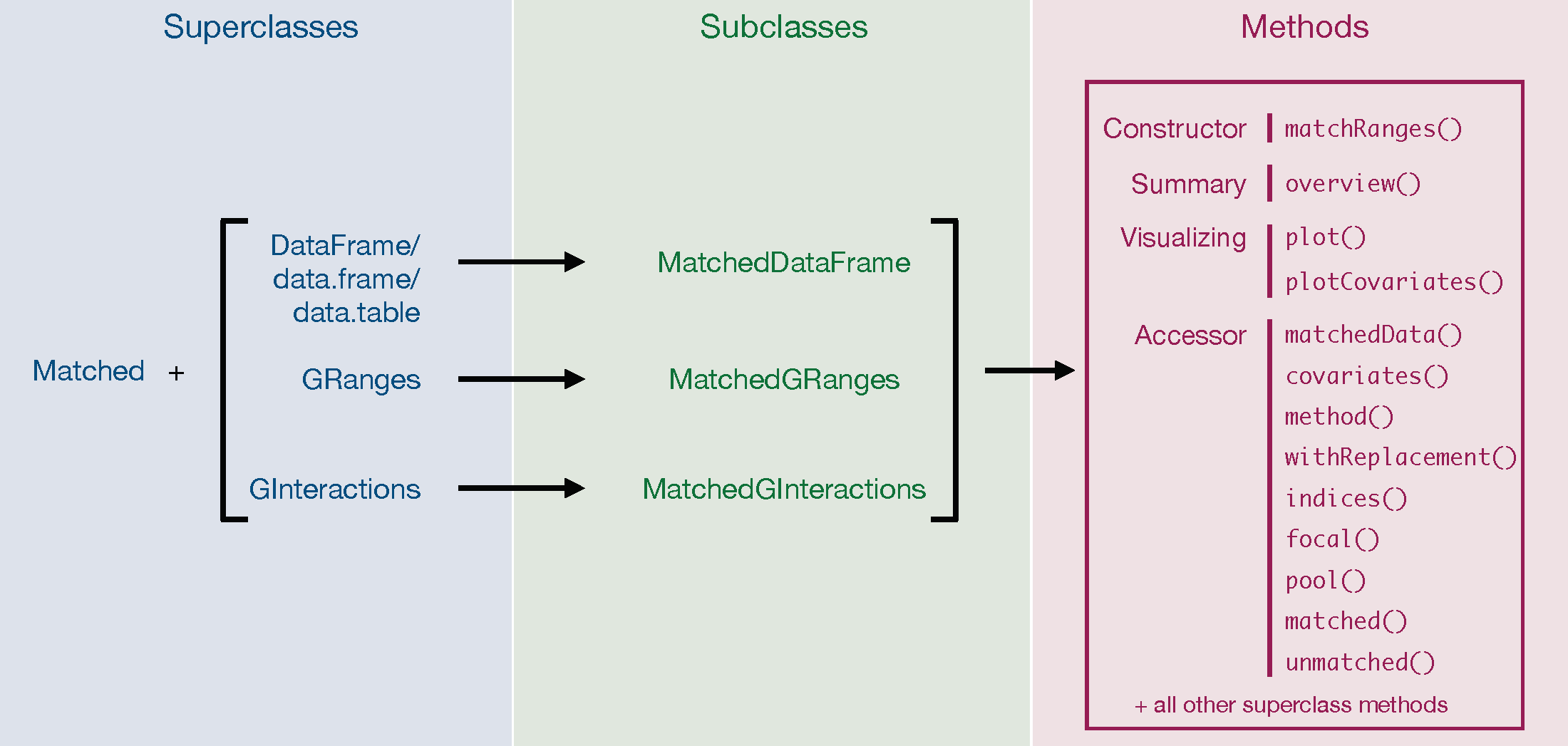
Internally, each Matched subclass uses a “delegate”
object of the same type to assign its slots. The delegate object used is
the matched set. Therefore, the resulting
Matched* object behaves as a combination of both its
superclasses - with access to methods from both.
For example, using matchRanges() on GRanges
objects assigns a GRanges delegate object which is used to
populate GRanges-specific slots. This results in a
MatchedGRanges object, with access to both
Matched functions (e.g. plotCovariate) as well
as normal GRanges methods (e.g.s seqnames,
resize, etc…).
Session information
## R version 4.5.2 (2025-10-31)
## Platform: x86_64-pc-linux-gnu
## Running under: Ubuntu 24.04.3 LTS
##
## Matrix products: default
## BLAS:   /usr/lib/x86_64-linux-gnu/openblas-pthread/libblas.so.3
## LAPACK: /usr/lib/x86_64-linux-gnu/openblas-pthread/libopenblasp-r0.3.26.so;  LAPACK version 3.12.0
##
## locale:
##  [1] LC_CTYPE=en_US.UTF-8       LC_NUMERIC=C
##  [3] LC_TIME=en_US.UTF-8        LC_COLLATE=en_US.UTF-8
##  [5] LC_MONETARY=en_US.UTF-8    LC_MESSAGES=en_US.UTF-8
##  [7] LC_PAPER=en_US.UTF-8       LC_NAME=C
##  [9] LC_ADDRESS=C               LC_TELEPHONE=C
## [11] LC_MEASUREMENT=en_US.UTF-8 LC_IDENTIFICATION=C
##
## time zone: UTC
## tzcode source: system (glibc)
##
## attached base packages:
## [1] stats4    grid      stats     graphics  grDevices utils     datasets
## [8] methods   base
##
## other attached packages:
##  [1] cobalt_4.6.1         plyranges_1.30.1     dplyr_1.1.4
##  [4] patchwork_1.3.2      GenomicRanges_1.62.0 Seqinfo_1.0.0
##  [7] IRanges_2.44.0       S4Vectors_0.48.0     BiocGenerics_0.56.0
## [10] generics_0.1.4       ggplot2_4.0.1        plotgardener_1.16.0
## [13] nullranges_1.17.3
##
## loaded via a namespace (and not attached):
##  [1] tidyselect_1.2.1            farver_2.1.2
##  [3] Biostrings_2.78.0           S7_0.2.1
##  [5] bitops_1.0-9                fastmap_1.2.0
##  [7] RCurl_1.98-1.17             pracma_2.4.6
##  [9] GenomicAlignments_1.46.0    XML_3.99-0.20
## [11] digest_0.6.39               lifecycle_1.0.4
## [13] magrittr_2.0.4              compiler_4.5.2
## [15] progress_1.2.3              rlang_1.1.6
## [17] sass_0.4.10                 tools_4.5.2
## [19] yaml_2.3.10                 data.table_1.17.8
## [21] rtracklayer_1.70.0          knitr_1.50
## [23] prettyunits_1.2.0           labeling_0.4.3
## [25] S4Arrays_1.10.0             htmlwidgets_1.6.4
## [27] mclust_6.1.2                curl_7.0.0
## [29] DelayedArray_0.36.0         RColorBrewer_1.1-3
## [31] KernSmooth_2.23-26          abind_1.4-8
## [33] BiocParallel_1.44.0         withr_3.0.2
## [35] purrr_1.2.0                 desc_1.4.3
## [37] Rhdf5lib_1.32.0             scales_1.4.0
## [39] ggridges_0.5.7              SummarizedExperiment_1.40.0
## [41] mvtnorm_1.3-3               cli_3.6.5
## [43] rmarkdown_2.30              crayon_1.5.3
## [45] ragg_1.5.0                  httr_1.4.7
## [47] rjson_0.2.23                cachem_1.1.0
## [49] rhdf5_2.54.0                parallel_4.5.2
## [51] ggplotify_0.1.3             XVector_0.50.0
## [53] restfulr_0.0.16             matrixStats_1.5.0
## [55] vctrs_0.6.5                 yulab.utils_0.2.1
## [57] Matrix_1.7-4                jsonlite_2.0.0
## [59] hms_1.1.4                   gridGraphics_0.5-1
## [61] systemfonts_1.3.1           strawr_0.0.92
## [63] jquerylib_0.1.4             glue_1.8.0
## [65] pkgdown_2.2.0               chk_0.10.0
## [67] codetools_0.2-20            gtable_0.3.6
## [69] GenomeInfoDb_1.46.0         BiocIO_1.20.0
## [71] UCSC.utils_1.6.0            tibble_3.3.0
## [73] pillar_1.11.1               rappdirs_0.3.3
## [75] htmltools_0.5.8.1           rhdf5filters_1.22.0
## [77] R6_2.6.1                    ks_1.15.1
## [79] textshaping_1.0.4           evaluate_1.0.5
## [81] lattice_0.22-7              Biobase_2.70.0
## [83] Rsamtools_2.26.0            cigarillo_1.0.0
## [85] bslib_0.9.0                 Rcpp_1.1.0
## [87] InteractionSet_1.38.0       SparseArray_1.10.1
## [89] xfun_0.54                   fs_1.6.6
## [91] MatrixGenerics_1.22.0       pkgconfig_2.0.3